Let’s visualize the Fibonnaci sequence
The Fibonacci sequence is one of the most famous and intriguing number sequences in mathematics. It is defined by a simple rule: Each number in the sequence is the sum of the two preceding numbers. The sequence starts with 0 and 1, and then each subsequent number is the sum of the previous two. So, the Fibonacci sequence looks like this:
0, 1, 1, 2, 3, 5, 8, 13, 21, 34, 55, ...
As the sequence progresses, the ratio of consecutive Fibonacci numbers approaches the famous golden ratio, approximately 1.61803398875. This ratio has fascinated mathematicians, artists, and scientists for centuries due to its remarkable properties.
Properties of the Fibonacci Sequence:
- Golden Ratio (Phi): As mentioned earlier, the ratio of consecutive Fibonacci numbers approaches the golden ratio (Phi), which is approximately 1.61803398875. The golden ratio has unique mathematical properties and is often found in nature, art, and architecture.
- Spiral Pattern: When the Fibonacci numbers are used to create a spiral, known as the Fibonacci spiral, it produces an aesthetically pleasing and naturally occurring spiral pattern. This spiral can be found in various natural phenomena like the arrangement of seeds in a sunflower, the curve of a nautilus shell, or the pattern of pinecones.
- Fibonacci Rectangles: The Fibonacci sequence is also related to a series of rectangles called Fibonacci rectangles. Each rectangle’s dimensions are consecutive Fibonacci numbers, and when they are combined, they create a logarithmic spiral.
- Fibonacci Tiling: When Fibonacci rectangles are used to tile a surface, they form a visually stunning and harmonious pattern called Fibonacci tiling. This tiling has been used in various artistic and architectural designs.
Relevance and Applications:
The Fibonacci sequence and the golden ratio have far-reaching implications across various disciplines:
- Art and Design: Many artists and designers use Fibonacci sequences and the golden ratio to create aesthetically pleasing compositions and designs. These concepts are often found in art, photography, and architecture.
- Financial Markets: The Fibonacci sequence is also used in financial markets, particularly in technical analysis, to identify potential support and resistance levels. Traders use Fibonacci retracement levels to predict potential market reversals.
- Computer Science: Fibonacci numbers have applications in computer algorithms, particularly in areas like dynamic programming and combinatorial optimization problems.
- Nature and Biology: The Fibonacci sequence is found in various aspects of the natural world, from the growth patterns of plants and the arrangement of leaves on stems to the spiral patterns of galaxies and hurricanes.
- Art and Design: Many artists and designers use Fibonacci sequences and the golden ratio to create aesthetically pleasing compositions and designs. These concepts are often found in art, photography, and architecture.
- Financial Markets: The Fibonacci sequence is used in financial markets, particularly in technical analysis, to identify potential support and resistance levels. Traders use Fibonacci retracement levels to predict potential market reversals.
- Computer Science: Fibonacci numbers have applications in computer algorithms, particularly in areas like dynamic programming and combinatorial optimization problems.
- Nature and Biology: The Fibonacci sequence is found in various aspects of the natural world, from the growth patterns of plants and the arrangement of leaves on stems to the spiral patterns of galaxies and hurricanes.
import pandas as pd
import matplotlib.pyplot as plt
import numpy as np

def generate_fibonacci_sequence(n):
    fib_sequence = [1.0, 1.0]
    while len(fib_sequence) < n:
        next_num = fib_sequence[-1] + fib_sequence[-2]
        fib_sequence.append(next_num)
    return fib_sequence

n = 40

fib_sequence = generate_fibonacci_sequence(n)
fib_df = pd.DataFrame(fib_sequence, columns=['fib_sequence'])
fib_df['Index'] = fib_df.index + 1
fib_df['Ratio'] = fib_df.fib_sequence / fib_df.fib_sequence.shift()
theta = 2 * np.pi * fib_df['Index'] / fib_df['Index'].max()
radius = np.log(fib_df.fib_sequence) * 2
fig, ax = plt.subplots(subplot_kw={'projection': 'polar'}, figsize=(15,15))
ax.plot(theta, radius, marker='o', linestyle='-', color='b', label='Fibonacci Numbers')
for i, row in fib_df.iterrows():
    ax.annotate(f'{int(row.fib_sequence)}', xy=(theta[i], radius[i]), xytext=(6, 6), textcoords='offset points')

ax.set_rticks([])
ax.set_title('Fibonacci Sequence')
ax.legend()
plt.show()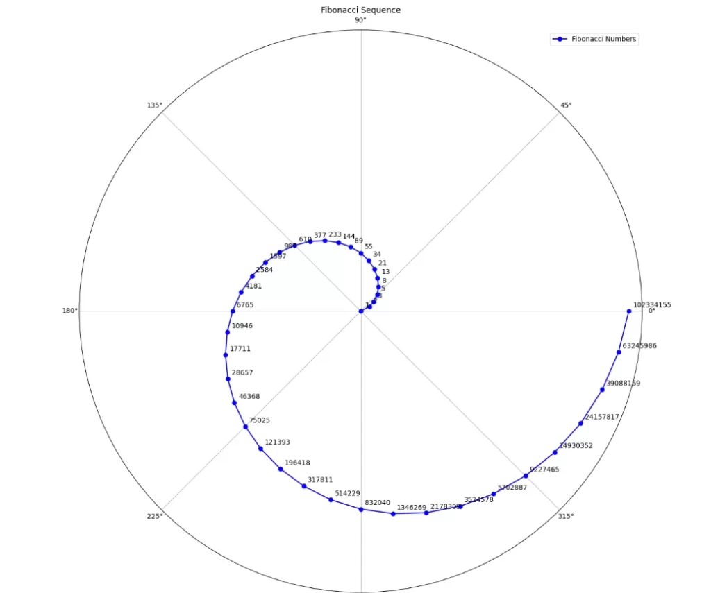
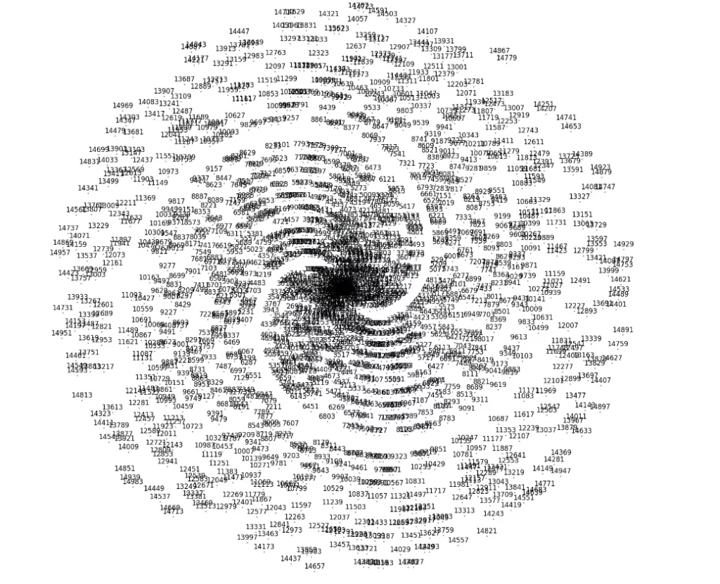
Prime Numbers
Prime numbers are fascinating and fundamental elements in number theory, possessing unique properties and significance in mathematics. A prime number is a positive integer greater than 1 that has no positive divisors other than 1 and itself. For example, 2, 3, 5, 7, 11, and 13 are prime numbers. The study of prime numbers has captivated mathematicians for centuries due to their mysterious and intriguing nature.
Properties of Prime Numbers
- Uniqueness: Every positive integer greater than 1 can be expressed as a unique product of prime numbers. This property is known as the Fundamental Theorem of Arithmetic. For example, the number 12 can be expressed as 2 * 2 * 3, where 2 and 3 are prime factors.
- Infinitude: There are infinitely many prime numbers. Euclid first proved this theorem around 300 BCE. The proof is elegant and shows that no matter how large a list of prime numbers we have, there will always be another prime number not in the list.
- Distribution: Prime numbers are not evenly distributed among all integers. As numbers get larger, prime numbers become rarer. However, there is no known formula to predict the exact position of the next prime number.
- Goldbach Conjecture: One of the oldest unsolved problems in number theory is the Goldbach Conjecture, which states that every even integer greater than 2 can be expressed as the sum of two prime numbers. Although this conjecture has been verified for large numbers, a formal proof remains elusive.
import math
import sympy

def get_coordinate(num):
    return num * np.cos(num), num * np.sin(num)

def create_plot(nums, figsize=20):
    nums = np.array(list(nums))
    x, y = get_coordinate(nums)
    plt.figure(figsize=(figsize, figsize))
    plt.axis("off")
    plt.scatter(x, y, s=1)
    for i, num in enumerate(nums):
        plt.annotate(num, (x[i], y[i]), textcoords="offset points", xytext=(0,5), ha='center', fontsize=12)

    plt.show()
primes = sympy.primerange(0, 15000)

create_plot(primes)
Number Theory Dataset: Exploring Properties of Numbers
Number theory is a branch of mathematics that deals with the properties of integers and their relationships. It is a fascinating area of study that has intrigued mathematicians for centuries. In this project, we will create a dataset that includes numbers and their properties related to number theory. We will explore various number properties, such as factors, divisors, multiples, and coprimes, using Python’s Pandas library. We will also visualize these properties to gain insights into number theory concepts.
Data Collection and Preparation
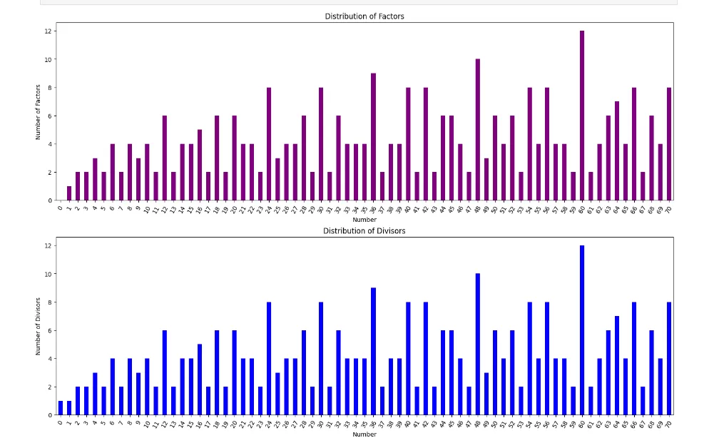
To create the Number Theory Dataset, we will generate a list of integers and compute their properties. For each number, we will calculate its factors, divisors, multiples, and coprimes. Here is a brief overview of these properties:
- Factors: Factors are the positive integers that divide a number without leaving a remainder. For example, the factors of 6 are 1, 2, 3, and 6.
- Divisors: Divisors are similar to factors but include negative integers as well. For example, the divisors of 6 are -6, -3, -2, -1, 1, 2, 3, and 6.
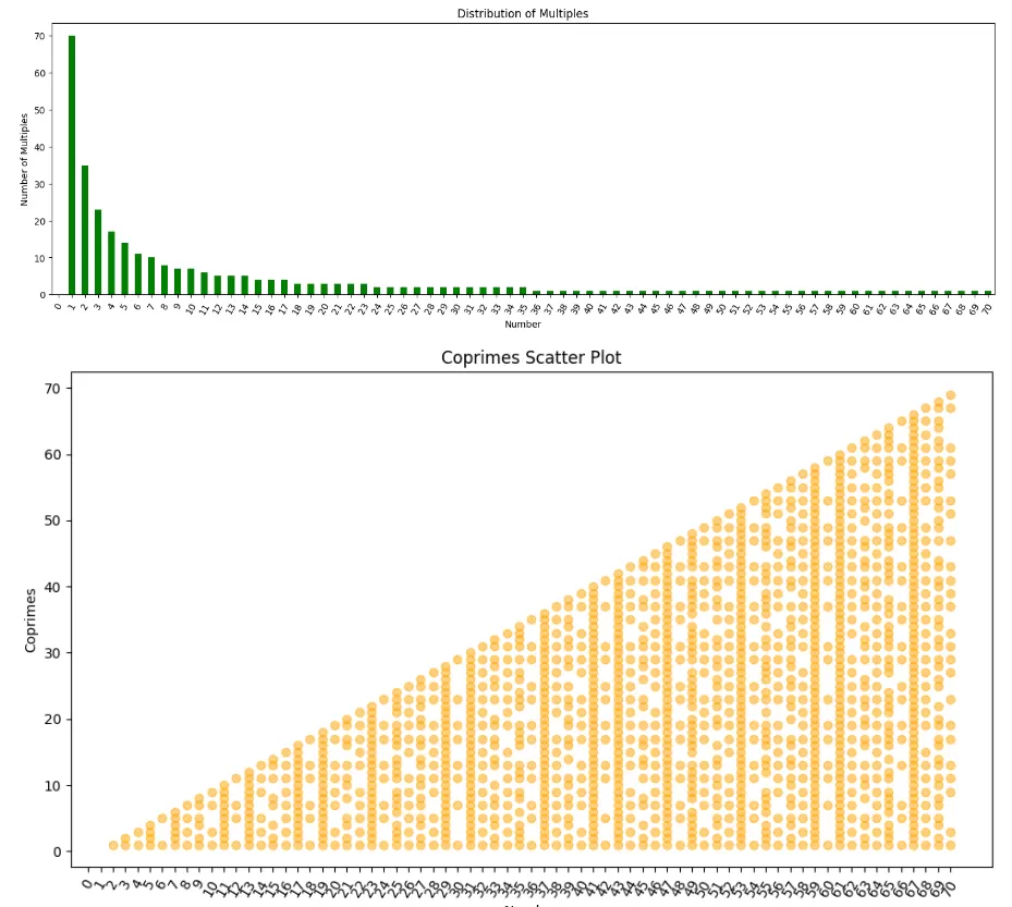
- Multiples: Multiples are the numbers that result from multiplying a number by other integers. For example, the multiples of 3 are 3, 6, 9, 12, and so on.
- Coprimes: Coprimes, also known as relatively prime numbers, are two numbers that have no common factors other than 1. For example, 9 and 16 are coprimes because they do not share any factors other than 1.
In [48]:
def factors(n):
    return [x for x in range(1, n+1) if n % x == 0]

def divisors(n):
    if n == 0:
        return [0]
    return [x for x in range(1, n+1) if n % x == 0]

def multiples(n, limit):
    if n == 0:
        return []
    return [x for x in range(n, limit+1, n)]

def coprimes(n):
    return [x for x in range(1, n) if np.gcd(n, x) == 1]

numbers = list(range(71))
df = pd.DataFrame({
    'Number': numbers,
    'Factors': [factors(num) for num in numbers],
    'Divisors': [divisors(num) for num in numbers],
    'Multiples': [multiples(num, 70) for num in numbers],
    'Coprimes': [coprimes(num) for num in numbers],
})

fig, axes = plt.subplots(3, 1, figsize=(15, 15))

df['Factors'].apply(len).plot(kind='bar', ax=axes[0], color='purple')
axes[0].set_title('Distribution of Factors')
axes[0].set_xlabel('Number')
axes[0].set_ylabel('Number of Factors')

df['Divisors'].apply(len).plot(kind='bar', ax=axes[1], color='blue')
axes[1].set_title('Distribution of Divisors')
axes[1].set_xlabel('Number')
axes[1].set_ylabel('Number of Divisors')

df['Multiples'].apply(len).plot(kind='bar', ax=axes[2], color='green')
axes[2].set_title('Distribution of Multiples')
axes[2].set_xlabel('Number')
axes[2].set_ylabel('Number of Multiples')

plt.tight_layout()

for ax in axes:
    ax.set_xticklabels(numbers, rotation=60)

plt.show()

plt.figure(figsize=(10, 6))
for i, row in df.iterrows():
    plt.scatter([row['Number']] * len(row['Coprimes']), row['Coprimes'], color='orange', alpha=0.5)
plt.title('Coprimes Scatter Plot')
plt.xlabel('Number')
plt.ylabel('Coprimes')
plt.xticks(numbers, rotation=60)
plt.tight_layout()
plt.show()
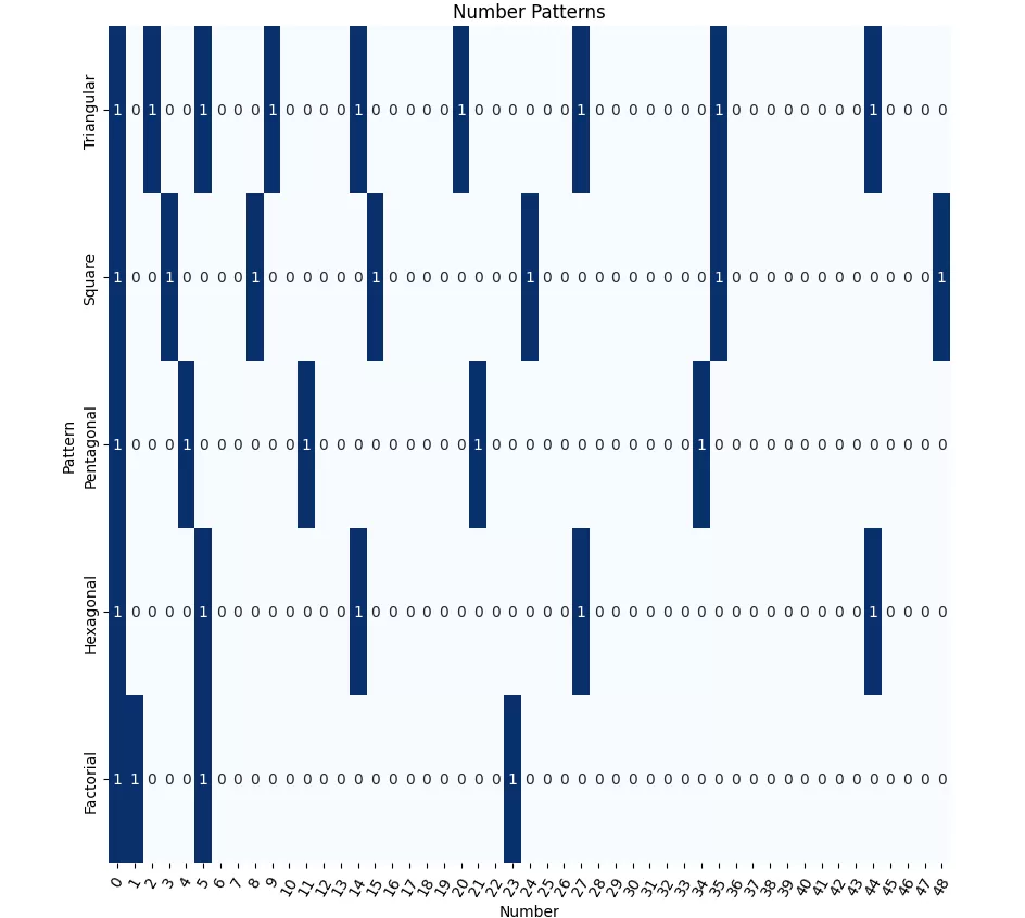
Number Patterns Dataset – Exploring Number Patterns with Pandas
In this analysis, we will generate a dataset that showcases various number patterns, such as triangular numbers, square numbers, pentagonal numbers, and more. We will then utilize the Pandas library to explore and visualize these fascinating number patterns.
- Triangular Numbers: Numbers that can be represented as equilateral triangles.
- Square Numbers: Numbers that are the squares of integers.
- Pentagonal Numbers: Numbers that can be represented as regular pentagons.
- Hexagonal Numbers: Numbers that can be represented as regular hexagons.
- Factorial Numbers: Numbers that are the products of all positive integers up to that number.
In [68]:
import seaborn as sns


def triangular_number(n):
    return (n * (n + 1)) // 2

def square_number(n):
    return n ** 2

def pentagonal_number(n):
    return (n * (3 * n - 1)) // 2

def hexagonal_number(n):
    return n * (2 * n - 1)

def factorial_number(n):
    if n == 0:
        return 1
    return n * factorial_number(n - 1) if n <= 20 else float('inf')
numbers = list(range(1, 50))

df = pd.DataFrame({
    'Number': numbers,
    'Triangular': [triangular_number(num) for num in numbers],
    'Square': [square_number(num) for num in numbers],
    'Pentagonal': [pentagonal_number(num) for num in numbers],
    'Hexagonal': [hexagonal_number(num) for num in numbers],
    'Factorial': [factorial_number(num) for num in numbers],
}
)
df['Triangular'] = df['Number'].apply(lambda x: 1 if x in df['Triangular'].values else 0)
df['Square'] = df['Number'].apply(lambda x: 1 if x in df['Square'].values else 0)
df['Pentagonal'] = df['Number'].apply(lambda x: 1 if x in df['Pentagonal'].values else 0)
df['Hexagonal'] = df['Number'].apply(lambda x: 1 if x in df['Hexagonal'].values else 0)
df['Factorial'] = df['Number'].apply(lambda x: 1 if x in df['Factorial'].values else 0)

df_heatmap = df.drop(columns='Number')

plt.figure(figsize=(10, 10))
sns.heatmap(df_heatmap.T, cmap='Blues', annot=True, fmt='g', cbar=False)
plt.xlabel('Number')
plt.ylabel('Pattern')
plt.title('Number Patterns')
plt.xticks(rotation=60)
plt.show()
Euler’s Totient Function, also known as the Phi function (often denoted as φ(n)), is an important concept in number theory. It is named after the Swiss mathematician Leonhard Euler, who introduced this function in the 18th century. The totient function is used to determine the count of positive integers that are relatively prime to a given positive integer n.
Two integers are considered relatively prime if their greatest common divisor (GCD) is 1. For example, the integers 8 and 15 are relatively prime because their GCD is 1 (gcd(8, 15) = 1), whereas the integers 12 and 18 are not relatively prime because their GCD is 6 (gcd(12, 18) = 6).
The value of φ(n) is the count of positive integers k (1 <= k <= n) that are relatively prime to n. In other words, φ(n) gives the number of positive integers less than or equal to n that share no common divisors with n (except for 1). If n is a prime number, then φ(n) is equal to n-1, as all numbers from 1 to n-1 will be relatively prime to n.
Calculation of Euler’s Totient Function (φ(n)):
To calculate φ(n) for a given positive integer n, we can follow these steps:
- Find the prime factors of n.
- For each prime factor p, subtract n/p from n (φ(n) = n – n/p).
- Repeat this process for all prime factors of n.
- The result is φ(n), the count of positive integers that are relatively prime to n.
In [77]:
import numpy as np
import matplotlib.pyplot as plt

def euler_totient_function(n):
    phi = n
    p = 2
    while p * p <= n:
        if n % p == 0:
            while n % p == 0:
                n //= p
            phi -= phi // p
        p += 1
    if n > 1:
        phi -= phi // n
    return phi

def generate_totient_data(n_range):
    numbers = list(range(1, n_range + 1))
    totient_values = [euler_totient_function(num) for num in numbers]
    return numbers, totient_values

def plot_totient_function(n_range):
    numbers, totient_values = generate_totient_data(n_range)
    plt.figure(figsize=(12, 6))
    plt.plot(numbers, totient_values, marker='o', color='blue')
    plt.xlabel('n')
    plt.ylabel('φ(n)')
    plt.title("Euler's Totient Function (φ(n))")
    plt.grid(True)
    plt.show()

plot_totient_function(120)
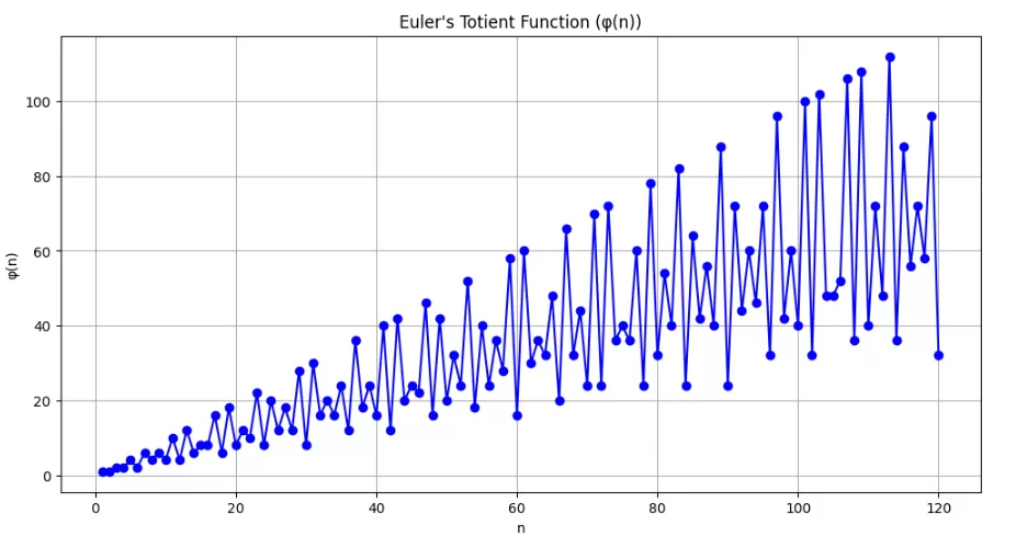
The pattern observed in the plot of Euler’s Totient Function (φ(n)) reveals some interesting insights about the distribution of relatively prime numbers and the behavior of the function:
- Cyclic Behavior: The plot exhibits a cyclic pattern, where the values of φ(n) rise and fall in a periodic manner. This cyclic behavior is due to the relationships between the prime factors of the numbers being considered. The function φ(n) is influenced by the prime factors of n, and as n varies, the presence or absence of specific prime factors leads to periodic changes in φ(n).
- High Values for Prime Numbers: For prime numbers (n = 2, 3, 5, 7, etc.), the value of φ(n) is equal to n-1. This is because all positive integers less than a prime number are relatively prime to it (gcd(k, n) = 1 for k = 1 to n-1). Therefore, φ(n) reaches its highest value when n is prime.
- Low Values for Composite Numbers: For composite numbers (non-prime numbers), the value of φ(n) is less than n-1. This is because composite numbers have common divisors with some positive integers less than n, reducing the count of relatively prime numbers. The more distinct prime factors a composite number has, the lower its φ(n) value.
- Relative Prime Pairs: The peaks in the plot represent numbers for which φ(n) is relatively high, indicating that these numbers have a significant number of relative prime pairs among the positive integers less than them. In contrast, the valleys in the plot correspond to numbers with relatively low φ(n) values, indicating a lower count of relative prime pairs.
- Asymptotic Growth: As n increases, φ(n) tends to grow asymptotically. This is because the number of positive integers that are relatively prime to n increases as n becomes larger. However, the rate of growth slows down as n grows, resulting in the cyclic pattern observed in the plot.
Overall, the plot of Euler’s Totient Function (φ(n)) provides valuable insights into the distribution of relatively prime numbers and the influence of prime factors on the number of relative prime pairs for each positive integer n. It highlights the cyclic nature of the function, with peaks at prime numbers and valleys at composite numbers. Additionally, the plot illustrates the overall increasing trend of φ(n) as n becomes larger. Euler’s Totient Function is a fundamental concept in number theory with applications in various fields, including cryptography and number theory algorithms.