Mathematics

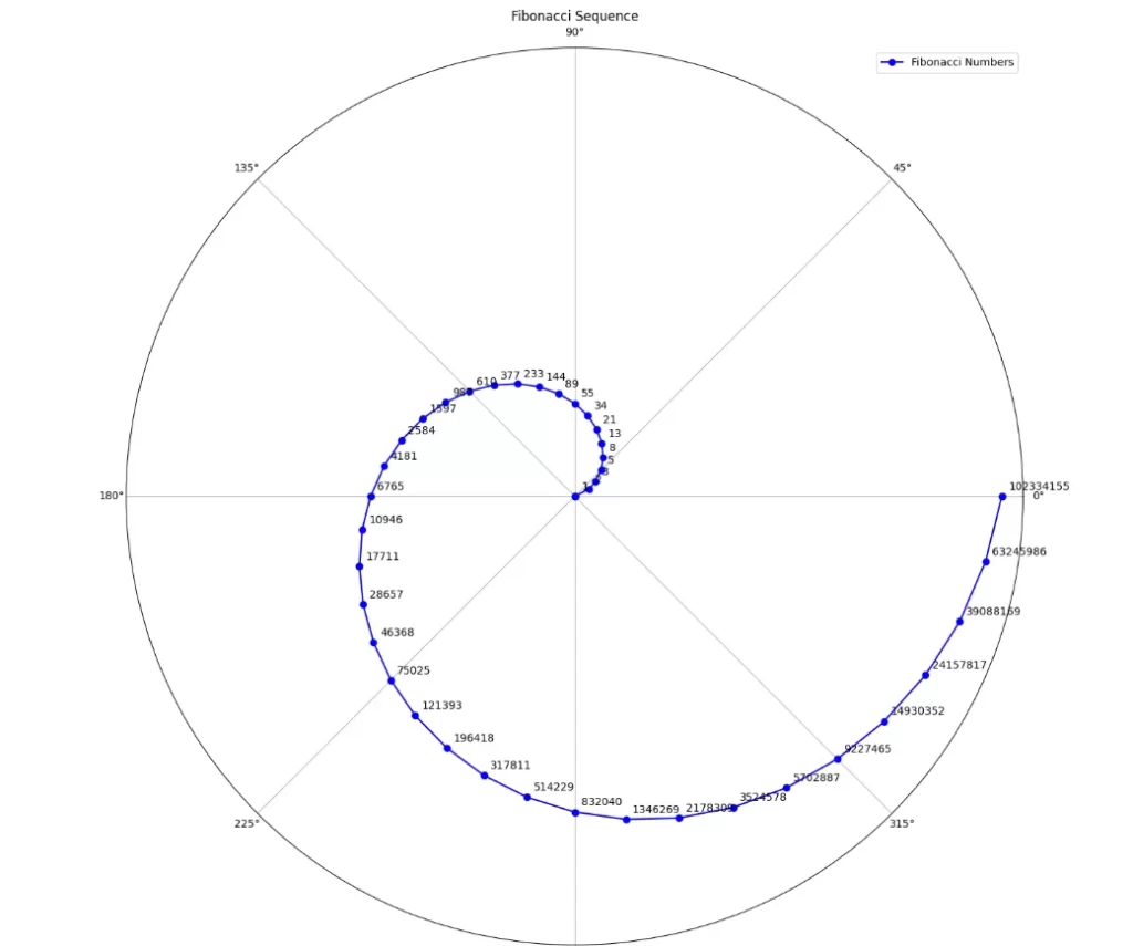
Let’s visualize the Fibonnaci sequence The Fibonacci sequence is one of the most famous and intriguing number sequences in mathematics. It is defined by a simple rule: Each number in the sequence is the sum of the two preceding numbers. The sequence starts with 0 and 1, and then each subsequent number is the sum of the previous two. So, the Fibonacci sequence looks like this: As the sequence progresses, the ratio of consecutive Fibonacci numbers approaches the famous golden ratio, approximately 1.61803398875. This ratio has fascinated mathematicians, artists, and scientists for centuries due to its remarkable properties. Properties of the Fibonacci Sequence: Relevance and Applications: The Fibonacci sequence and the golden ratio have far-reaching implications across various disciplines: Prime Numbers Prime numbers are fascinating and fundamental elements in number theory, possessing unique properties and significance in mathematics. A prime number is a positive integer greater than 1 that has no positive divisors other than 1 and itself. For example, 2, 3, 5, 7, 11, and 13 are prime numbers. The study of prime numbers has captivated mathematicians for centuries due to their mysterious and intriguing nature. Properties of Prime Numbers import math import sympy def get_coordinate(num): return num * np.cos(num), num * np.sin(num) def create_plot(nums, figsize=20): nums = np.array(list(nums)) x, y = get_coordinate(nums) plt.figure(figsize=(figsize, figsize)) plt.axis(“off”) plt.scatter(x, y, s=1) for i, num in enumerate(nums): plt.annotate(num, (x[i], y[i]), textcoords=”offset points”, xytext=(0,5), ha=’center’, fontsize=12) plt.show() primes = sympy.primerange(0, 15000) create_plot(primes) Number Theory Dataset: Exploring Properties of Numbers Number theory is a branch of mathematics that deals with the properties of integers and their relationships. It is a fascinating area of study that has intrigued mathematicians for centuries. In this project, we will create a dataset that includes numbers and their properties related to number theory. We will explore various number properties, such as factors, divisors, multiples, and coprimes, using Python’s Pandas library. We will also visualize these properties to gain insights into number theory concepts. Data Collection and Preparation To create the Number Theory Dataset, we will generate a list of integers and compute their properties. For each number, we will calculate its factors, divisors, multiples, and coprimes. Here is a brief overview of these properties: In [48]: def factors(n): return [x for x in range(1, n+1) if n % x == 0] def divisors(n): if n == 0: return [0] return [x for x in range(1, n+1) if n % x == 0] def multiples(n, limit): if n == 0: return [] return [x for x in range(n, limit+1, n)] def coprimes(n): return [x for x in range(1, n) if np.gcd(n, x) == 1] numbers = list(range(71)) df = pd.DataFrame({ ‘Number’: numbers, ‘Factors’: [factors(num) for num in numbers], ‘Divisors’: [divisors(num) for num in numbers], ‘Multiples’: [multiples(num, 70) for num in numbers], ‘Coprimes’: [coprimes(num) for num in numbers], }) fig, axes = plt.subplots(3, 1, figsize=(15, 15)) df[‘Factors’].apply(len).plot(kind=’bar’, ax=axes[0], color=’purple’) axes[0].set_title(‘Distribution of Factors’) axes[0].set_xlabel(‘Number’) axes[0].set_ylabel(‘Number of Factors’) df[‘Divisors’].apply(len).plot(kind=’bar’, ax=axes[1], color=’blue’) axes[1].set_title(‘Distribution of Divisors’) axes[1].set_xlabel(‘Number’) axes[1].set_ylabel(‘Number of Divisors’) df[‘Multiples’].apply(len).plot(kind=’bar’, ax=axes[2], color=’green’) axes[2].set_title(‘Distribution of Multiples’) axes[2].set_xlabel(‘Number’) axes[2].set_ylabel(‘Number of Multiples’) plt.tight_layout() for ax in axes: ax.set_xticklabels(numbers, rotation=60) plt.show() plt.figure(figsize=(10, 6)) for i, row in df.iterrows(): plt.scatter([row[‘Number’]] * len(row[‘Coprimes’]), row[‘Coprimes’], color=’orange’, alpha=0.5) plt.title(‘Coprimes Scatter Plot’) plt.xlabel(‘Number’) plt.ylabel(‘Coprimes’) plt.xticks(numbers, rotation=60) plt.tight_layout() plt.show() Number Patterns Dataset – Exploring Number Patterns with Pandas In this analysis, we will generate a dataset that showcases various number patterns, such as triangular numbers, square numbers, pentagonal numbers, and more. We will then utilize the Pandas library to explore and visualize these fascinating number patterns. In [68]: import seaborn as sns def triangular_number(n): return (n * (n + 1)) // 2 def square_number(n): return n ** 2 def pentagonal_number(n): return (n * (3 * n – 1)) // 2 def hexagonal_number(n): return n * (2 * n – 1) def factorial_number(n): if n == 0: return 1 return n * factorial_number(n – 1) if n <= 20 else float(‘inf’) numbers = list(range(1, 50)) df = pd.DataFrame({ ‘Number’: numbers, ‘Triangular’: [triangular_number(num) for num in numbers], ‘Square’: [square_number(num) for num in numbers], ‘Pentagonal’: [pentagonal_number(num) for num in numbers], ‘Hexagonal’: [hexagonal_number(num) for num in numbers], ‘Factorial’: [factorial_number(num) for num in numbers], } ) df[‘Triangular’] = df[‘Number’].apply(lambda x: 1 if x in df[‘Triangular’].values else 0) df[‘Square’] = df[‘Number’].apply(lambda x: 1 if x in df[‘Square’].values else 0) df[‘Pentagonal’] = df[‘Number’].apply(lambda x: 1 if x in df[‘Pentagonal’].values else 0) df[‘Hexagonal’] = df[‘Number’].apply(lambda x: 1 if x in df[‘Hexagonal’].values else 0) df[‘Factorial’] = df[‘Number’].apply(lambda x: 1 if x in df[‘Factorial’].values else 0) df_heatmap = df.drop(columns=’Number’) plt.figure(figsize=(10, 10)) sns.heatmap(df_heatmap.T, cmap=’Blues’, annot=True, fmt=’g’, cbar=False) plt.xlabel(‘Number’) plt.ylabel(‘Pattern’) plt.title(‘Number Patterns’) plt.xticks(rotation=60) plt.show() Euler’s Totient Function, also known as the Phi function (often denoted as φ(n)), is an important concept in number theory. It is named after the Swiss mathematician Leonhard Euler, who introduced this function in the 18th century. The totient function is used to determine the count of positive integers that are relatively prime to a given positive integer n. Two integers are considered relatively prime if their greatest common divisor (GCD) is 1. For example, the integers 8 and 15 are relatively prime because their GCD is 1 (gcd(8, 15) = 1), whereas the integers 12 and 18 are not relatively prime because their GCD is 6 (gcd(12, 18) = 6). The value of φ(n) is the count of positive integers k (1 <= k <= n) that are relatively prime to n. In other words, φ(n) gives the number of positive integers less than or equal to n that share no common divisors with n (except for 1). If n is a prime number, then φ(n) is equal to n-1, as all numbers from 1 to n-1 will be relatively prime to n. Calculation of Euler’s Totient Function (φ(n)): To calculate φ(n) for a given positive integer n, we can follow these steps: In [77]: import numpy as np import matplotlib.pyplot as plt def euler_totient_function(n): phi = n p = 2 while p * p <= n: if n % p == 0: while n % p == 0: n //= p phi